深度学习二:linear regression练习
前言
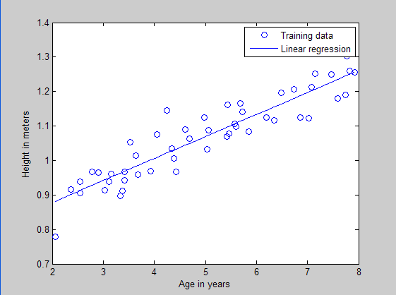
本文是多元线性回归的练习,这里练习的是最简单的二元线性回归,参考斯坦福大学的教学网http://openclassroom.stanford.edu/MainFolder/DocumentPage.php?course=DeepLearning&doc=exercises/ex2/ex2.html。本题给出的是50个数据样本点,其中x为这50个小朋友到的年龄,年龄为2岁到8岁,年龄可有小数形式呈现。Y为这50个小朋友对应的身高,当然也是小数形式表示的。现在的问题是要根据这50个训练样本,估计出3.5岁和7岁时小孩子的身高。通过画出训练样本点的分布凭直觉可以发现这是一个典型的线性回归问题。
matlab函数介绍:
legend:
比如legend('Training data', 'Linear regression'),它表示的是标出图像中各曲线标志所代表的意义,这里图像的第一条曲线(其实是离散的点)表示的是训练样本数据,第二条曲线(其实是一条直线)表示的是回归曲线。
hold on, hold off:
hold on指在前一幅图的情况下打开画纸,允许在上面继续画曲线。hold off指关闭前一副画的画纸。
linspace:
比如linspace(-3, 3, 100)指的是给出-3到3之间的100个数,均匀的选取,即线性的选取。
logspace:
比如logspace(-2, 2, 15),指的是在10^(-2)到10^(2)之间选取15个数,这些数按照指数大小来选取,即指数部分是均匀选取的,但是由于都取了10为底的指数,所以最终是服从指数分布选取的。
实验结果:
训练样本散点和回归曲线预测图:
损失函数与参数之间的曲面图:

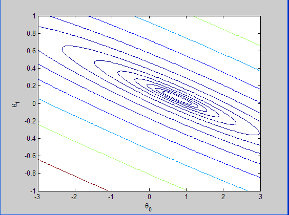
损失函数的等高线图:
程序代码及注释:
采用normal equations方法求解:
%%方法一
x = load('ex2x.dat');
y = load('ex2y.dat');
plot(x,y,'*')
xlabel('height')
ylabel('age')
x = [ones(size(x),1),x];
w=inv(x'*x)*x'*y
hold on
%plot(x,0.0639*x+0.7502)
plot(x(:,2),0.0639*x(:,2)+0.7502)%更正后的代码
采用gradient descend过程求解:
% Exercise 2 Linear Regression

% Data is roughly based on 2000 CDC growth figures
% for boys
%
% x refers to a boy's age
% y is a boy's height in meters
%

clear all; close all; clc
x = load('ex2x.dat'); y = load('ex2y.dat');

m = length(y); % number of training examples


% Plot the training data
figure; % open a new figure window
plot(x, y, 'o');
ylabel('Height in meters')
xlabel('Age in years')

% Gradient descent
x = [ones(m, 1) x]; % Add a column of ones to x
theta = zeros(size(x(1,:)))'; % initialize fitting parameters
MAX_ITR = 1500;
alpha = 0.07;

for num_iterations = 1:MAX_ITR
    % This is a vectorized version of the
    % gradient descent update formula
    % It's also fine to use the summation formula from the videos

    % Here is the gradient
    grad = (1/m).* x' * ((x * theta) - y);

    % Here is the actual update
    theta = theta - alpha .* grad;

    % Sequential update: The wrong way to do gradient descent
    % grad1 = (1/m).* x(:,1)' * ((x * theta) - y);
    % theta(1) = theta(1) + alpha*grad1;
    % grad2 = (1/m).* x(:,2)' * ((x * theta) - y);
    % theta(2) = theta(2) + alpha*grad2;
end
% print theta to screen
theta

% Plot the linear fit
hold on; % keep previous plot visible
plot(x(:,2), x*theta, '-')
legend('Training data', 'Linear regression')%标出图像中各曲线标志所代表的意义
hold off % don't overlay any more plots on this figure,指关掉前面的那幅图

% Closed form solution for reference
% You will learn about this method in future videos
exact_theta = (x' * x)\x' * y

% Predict values for age 3.5 and 7
predict1 = [1, 3.5] *theta
predict2 = [1, 7] * theta


% Calculate J matrix

% Grid over which we will calculate J
theta0_vals = linspace(-3, 3, 100);
theta1_vals = linspace(-1, 1, 100);

% initialize J_vals to a matrix of 0's
J_vals = zeros(length(theta0_vals), length(theta1_vals));

for i = 1:length(theta0_vals)
      for j = 1:length(theta1_vals)
      t = [theta0_vals(i); theta1_vals(j)];
      J_vals(i,j) = (0.5/m) .* (x * t - y)' * (x * t - y);
    end
end

% Because of the way meshgrids work in the surf command, we need to
% transpose J_vals before calling surf, or else the axes will be flipped
J_vals = J_vals';
% Surface plot
figure;
surf(theta0_vals, theta1_vals, J_vals)
xlabel('\theta_0'); ylabel('\theta_1');

% Contour plot
figure;
% Plot J_vals as 15 contours spaced logarithmically between 0.01 and 100
contour(theta0_vals, theta1_vals, J_vals, logspace(-2, 2, 15))%画出等高线
xlabel('\theta_0'); ylabel('\theta_1');%类似于转义字符,但是最多只能是到参数0~9
参考资料:
作者:tornadomeet
出处:http://www.cnblogs.com/tornadomeet 欢迎转载或分享,但请务必声明文章出处。


